2022/05/09 誤字修正、インストール手順修正(ggplot)
2022/06/09 heatmapのコマンド修正. 10/24 インストール手順修正(Rのバージョン4指定)
2023/06/18 追記
2024/02/27 docker image例追記
比較ハイスループットシーケンスアッセイでは、RNA-seqにおける遺伝子ごとのリードカウントのようなカウントデータを解析し、実験条件間での系統的変化の証拠を得ることが基本的なタスクとなる。小さな複製数、離散性、大きなダイナミックレンジ、および外れ値の存在には、適切な統計的アプローチが必要になる。この論文では、分散とフォールドチェンジの収縮推定を使用して、推定値の安定性と解釈可能性を向上させた、カウントデータの差分解析手法であるDESeq2を紹介する。これにより、単なる発現差の存在ではなく、その強さに焦点を当てたより定量的な解析が可能になる。DESeq2パッケージは、http://www.bioconductor.org/packages/release/bioc/html/DESeq2.html webciteで入手できる。
Doumentaion
http://bioconductor.org/packages/devel/bioc/vignettes/DESeq2/inst/doc/DESeq2.html#quick-start
https://bioc.ism.ac.jp/packages/2.14/bioc/vignettes/DESeq2/inst/doc/beginner.pdf
インストール
condaで環境を作って導入し、rstudioを使ってテストした(macos Monterey使用)。
#conda(link)
mamba create -n deseq2 python=3.9 -y
conda activate deseq2
mamba install -c conda-forge -c bioconda bioconductor-deseq2 -y
#R
mamba install -c conda-forge r-base=4 -y
#ggplot2 (link)
mamba install -c conda-forge r-ggplot2 -y
#rstudio
mamba install -c r rstudio -y

#BiocManager
if (!require("BiocManager", quietly = TRUE))
    install.packages("BiocManager")
BiocManager::install("DESeq2")

#Error: package or namespace load failed for ‘DESeq2’:
#package ‘DBI’ was installed before R 4.0.0: please re-install it が出たら、Rコンソールで再導入する
install.packages("DBI")
install.packages("httr")

#人気のdocker iamge (dockerhub)注;ggplotは含まれていない
docker run --rm -it -v $PWD:/data -w /data pegi3s/r_deseq2
> R #立ち上げ(イメージ作成者はRscriptとして外から実行することを推奨されている)
実行方法
ここではDESeq2の基本的な差分発現解析の流れを確認します。
生の整数リードカウントファイルを用意する。
1、ライブラリのロードとリードカウントファイルの読み込み
library("DESeq2")
library("ggplot2")

#tab区切りリードカウントマトリックスの読み込み
count <- read.table("count.txt",sep = "\t", header = T, row.names = 1)
head(count)
出力
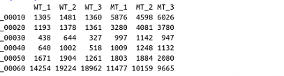
WT3反復、MT3反復の実験となっている。サンプル名はこの後利用するので、扱いやすい名前が望ましい。
2、DESeqのランにはサンプルグループについてのメタデータが必要。
data.frameの作成。data.frame() 関数を使う。sample名はステップ1のファイルのヘッダー名と一致している必要がある。
coldata <- data.frame(
sample = c("WT_1", "WT_2", "WT_3", "MT_1", "MT_2", "MT_3"),
condition = c("control", "control", "control", "treatment", "treatment", "treatment"),
row.names = "sample" )
3、DGE解析のためのDESeqDataSetオブジェクトを構築。DESeqDataSetFromMatrix関数(link)を使う(DESeqDataSet は 差分発現解析の入力値、中間計算、結果を格納するために使用される)。
dds <- DESeqDataSetFromMatrix(countData = count, colData = coldata, design = ~ condition)

#カウントデータは正の整数である必要がある。少数点以下があるなら丸める。
dds <- DESeqDataSetFromMatrix(countData = round(count), colData = coldata, design = ~ condition)
- countData for matrix input: a matrix of non-negative integers
- coldata for matrix input: a DataFrame or data.frame with at least a single column. Rows of colData correspond to columns of countData
- design a formula which expresses how the counts for each gene depend on the variables in colData. Many R formula are valid, including designs with multiple variables, e.g., ~ group + condition, and designs with interactions, e.g., ~ genotype + treatment + genotype:treatment. See results for a variety of designs and how to extract results tables. By default, the functions in this package will use the last variable in the formula for building results tables and plotting. ~ 1 can be used for no design, although users need to remember to switch to another design for differential testing.
4、リードカウントがゼロ近い遺伝子をフィルタリング
#全サンプルで合計10リード未満の遺伝子をフィルタリング
dds <- dds[rowSums(counts(dds)) >= 10,]
ddsデータオブジェクトのメモリサイズを削減し、計算を高速化する。マニュアルではリード数10を例としている。より厳密なフィルタリングは、主観で決めるのではなく、results関数内で正規化されたカウントの平均値に対するフィルタリングによって自動適用される。
5、リファレンスを選択(conditionで指定したグループ名)。他のコンディションの比較は、この ref 値を基準に比較される。ここではグループ;controlをリファレンスとして比較する。
dds$condition <- relevel(dds$condition, ref = "control")
このパラメータを設定しない場合、アルファベット順で比較される。
6、遺伝子発現の差分解析を行う。DESeq関数(link)を使う。
dds <- DESeq(dds)
出力
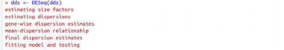
この関数は、サイズファクタの推定、分散の推定、負の二項GLMフィッティングとWald統計によってデフォルトの解析を行う。利用可能なオプションは”?DESeq”をタイプしても表示できる(link)。
=========補足==========================================
DESeq関数は以下の関数を順番に実行している
dds <- estimateSizeFactors(dds) #sizeFactorsの推定
dds <- estimateDispersions(dds) 負の二項分布のデータに対する分散推定値を求める
dds <- nbinomWaldTest(dds) #計算したsizeFactorsと分散推定値を用いて、Negative Binomial GLMにおける係数の有意性を検定
======================================================
resultsNamesはモデルの推定効果(係数)の名前を全比較に対して返す(ここでは1組のみ)。
resultsNames(dds)
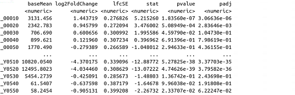
7、DESeq関数がDESeqDataSetオブジェクトを返した後、results関数(link)で結果表(log2 fold changeとp値)を抽出できる。
res <- results(dds)
res
results関数は、DESeq解析から、サンプル間の基本平均、log2 fold change、標準誤差、検定統計量、p値、adjusted p値を与える結果表を抽出する。
出力
関数plotMAは、DESeqDataSet内のすべてのサンプルについてlog2倍率変化のMA plotを表示する。
plotMA(res, ylim=c(-10,10))

#PDF保存
pdf("MA_plot.pdf")
plotMA(res, ylim=c(-10,10))
dev.off()
修正p値が0.1より小さい場合、ポイントは青色になる。指定幅以上(ここでは-5,+5)の対数倍率変化をしている遺伝子のポイントは三角形のプロットになる。
8、遺伝子発現表を調整済みp値(Benjamini-Hochberg FDR法)順に並べる。
res[order(res$padj),]
9、遺伝子発現差解析表をCSVファイルに書き出す(FDR順)。
write.csv(as.data.frame(res[order(res$padj),] ), file="output.csv")
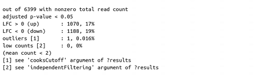
10、summary関数(link)を使って遺伝子発現の差の要約を表示。p値0.05でカットオフする。
summary(results(dds, alpha=0.05))
- alpha the adjusted p-value cutoff. if not set, this defaults to the alpha argument which was used in results to set the target FDR for independent filtering.
出力
11、正規化されたカウントを取得
normalized_counts <- counts(dds, normalized=TRUE)
head(normalized_counts)

#書き出し
write.csv(as.data.frame(normalized_counts), file="normalized_counts.csv")
12、オプションの解析
サンプル間距離のヒートマップ
#対数変換してDESeqTransformオブジェクトを作成(link)
ntd <- normTransform(dds)

#変換後のデータの標準偏差を、平均値に対してサンプル数でプロット
library("vsn") #link
meanSdPlot(assay(ntd))
分散推定値のプロット
plotDispEsts(dds)

sampleDists <- dist(t(assay(ntd)))
library("RColorBrewer")
library("pheatmap")
sampleDistMatrix <- as.matrix(sampleDists)

rownames(sampleDistMatrix) <- paste(ntd$condition, ntd$type, sep="-")
colnames(sampleDistMatrix) <- NULL
colors <- colorRampPalette(rev(brewer.pal(9, "Blues")))(255)
pdf("sample_distance_heatmap.pdf", width=7, height=7)
pheatmap(sampleDistMatrix,
         clustering_distance_rows = sampleDists,
         clustering_distance_cols = sampleDists,
         col = colors)
dev.off()

PCA plot
plotPCA(ntd, intgroup=c("condition"))

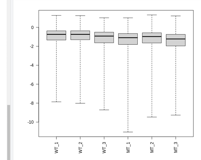
box plot
par(mar=c(8,5,2,2)) #余白調整
boxplot(log10(assays(dds)"cooks"), range=0, las=2)
引用
Moderated estimation of fold change and dispersion for RNA-seq data with DESeq2
Michael I Love, Wolfgang Huber, Simon Anders
Genome Biol. 2014;15(12):550
Differential expression analysis for sequence count data
Simon Anders & Wolfgang Huber
Genome Biology volume 11, Article number: R106 (2010)
参考
関連
参考
When NOT to use DESeq2 for RNA-seq analysis?
— Ming "Tommy" Tang (@tangming2005) January 22, 2025
DESeq2 is the gold standard for bulk RNA-seq, but it has limitations. If you’re analyzing large datasets, beware of inflated false discovery rates (FDR). 🧵👇