macでインフォマティクス

macでインフォマティクス

HTS (NGS) 関連のインフォマティクス情報についてまとめています。

K-mer分析ツール KAT

2019 5/15 リンク、condaインストール追加

2019 5/16  タイトル修正

2020 9/27 help更新


ハイスループットの全ゲノムショットガン(WGS)データセットの迅速な解析は、大きなサイズが生み出す複雑さのためにチャレンジングである(Schatz et al、2012)。 WGSデータを分析するためのリファレンスが不要なアプローチは、基本的な品質、リード長、GCコンテンツ(Yang et al、2013)の調査とk-mer(サイズk のワード)スペクトラム探索を含む(Chor et al、2009; Lo and Chain、2014)。頻繁に使用されるリファレンスフリーの品質管理ツールはFastQC(http://www.bioinformatics.babraham.ac.uk/projects/fastqc/)である。

K-merスペクトラムは、データ品質(エラーのレベル、シーケンシングバイアス、シーケンシングカバレッジおよび潜在的汚染)だけでなく、ゲノムの複雑さ(サイズ、核型、ヘテロ接合性および反復含有量; Simpson、2014)に関する情報を明らかにする。 WGSデータセットのペアワイズ比較(Anvar et al、2014)により、スペクトラムの違いを強調して問題のあるサンプルを識別できる追加情報を抽出できる。

K-mer analysis Tookitは、シーケンスデータから直接的に任意の長さのk-merのスペクトルを迅速にカウント、比較、分析するためのツール群である。任意の分布のk-merをフィルタリングする機能も備えている。


KAT's Documentation

Welcome to KAT’s documentation! — kat 2.4.1 documentation


f:id:kazumaxneo:20180501115728j:plain

マニュアルより転載。k-merスペクトラムを描くことで、ゲノムに関する様々な情報を得ることができる。図にはないが、たいていのシーケンスデータでは左端に最も大きいピークがある(おそらくシーケンスエラー由来)。


kat-comp introduction


k-mer counting, part I: Introduction


インストール

依存

  • GCC V4.8+
  • make
  • autoconf V2.53+
  • automake V1.11+
  • libtool V2.4.2+
  • pthreads (probably already installed)
  • zlib
  • Python V3.5+ with the tabulate, scipy, numpy and matplotlib packages and C API installed. Python is optional but highly recommended, without python, KAT functionality is limited: no plots, no distribution analysis, and no documentation.
  • Sphinx-doc V1.3+ (Optional: only required for building the documentation.

Github

https://github.com/TGAC/KAT

ビルドはやや複雑だが、KATはbrewによるインストールがサポートされており、ワンライナーで導入できる。

brew install brewsci/bio/kat

#bioconda
conda install -c bioconda -y kat

$ kat

The K-mer Analysis Toolkit (KAT) contains a number of tools that analyse jellyfish K-mer hashes. 


The First argument should be the tool/mode you wish to use:


   * hist:   Create an histogram of k-mer occurrences from a sequence file.  Similar to

             jellyfish histogram sub command but adds metadata in output for easy plotting,

             also actually runs multi-threaded.

   * gcp:    K-mer GC Processor.  Creates a matrix of the number of K-mers found given a GC

             count and a K-mer count.

   * comp:   K-mer comparison tool.  Creates a matrix of shared K-mers between two (or three)

             sequence files.

   * sect:   SEquence Coverage estimator Tool.  Estimates the coverage of each sequence in

             a file using K-mers from another sequence file.

   * cold:   Given, reads and an assembly, calculates both the read and assembly K-mer

             coverage along with GC% for each sequence in the assembly.

             a file using K-mers from another sequence file.

   * filter: Filtering tools.  Contains tools for filtering k-mers and sequences based on

             user-defined GC and coverage limits.

   * plot:   Plotting tools.  Contains several plotting tools to visualise K-mer and compare

             distributions.


Options:

  -v [ --verbose ]      Print extra information

  --version             Print version string

  --help                Produce help message


ラン

hist:  histogram of k-mer occurrences.

> kat hist

$ kat hist

Kmer Analysis Toolkit (KAT) V2.4.2


Usage: kat hist [options] (<input>)+


Create an histogram of k-mer occurrences from the input.


Create an histogram with the number of k-mers having a given count, derived from the input, which can take the form of a single jellyfish hash, or one or more FastA or FastQ files. In bucket 'i' are tallied the k-mers which have a count 'c' satisfying 'low+i*inc <= c < low+(i+1)'. Buckets in the output are labeled by the low end point (low+i).

The last bucket in the output behaves as a catchall: it tallies all k-mers with a count greater or equal to the low end point of this bucket.

This tool is very similar to the "histo" tool in jellyfish itself.  The primary difference being that the output contains metadata that make the histogram easier for the user to plot.


Options:

  -o [ --output_prefix ] arg (="kat.hist") Path prefix for files generated by this program.

  -t [ --threads ] arg (=1)                The number of threads to use

  -l [ --low ] arg (=1)                    Low count value of histogram

  -h [ --high ] arg (=10000)               High count value of histogram

  -i [ --inc ] arg (=1)                    Increment for each bin

  --5ptrim arg (=0)                        Ignore the first X bases from reads.  If more that one file is provided you can specify different values for each file by 

                                           seperating with commas.

  -N [ --non_canonical ]                   If counting fast(a/q), store explicit kmer as found.  By default, we store 'canonical' k-mers, which means we count both strands.

  -m [ --mer_len ] arg (=27)               The kmer length to use in the kmer hashes.  Larger values will provide more discriminating power between kmers but at the expense 

                                           of additional memory and lower coverage.

  -H [ --hash_size ] arg (=100000000)      If kmer counting is required for the input, then use this value as the hash size.  If this hash size is not large enough for your 

                                           dataset then the default behaviour is to double the size of the hash and recount, which will increase runtime and memory usage.

  -d [ --dump_hash ]                       Dumps any jellyfish hashes to disk that were produced during this run. Normally, this is not recommended, as hashes are slow to 

                                           load and will likely consume a significant amount of disk space.

  -p [ --output_type ] arg (=png)          The plot file type to create: png, ps, pdf.

  -v [ --verbose ]                         Print extra information.

  --help                                   Produce help message.


k-merサイズ27でペアエンドのfastqを分析。横軸の最大値は10000とする。

kat hist -t 8 -l 1 -h 10000 -m 27 -v -o output sample1_*.fastq

頻度を示したテキストファイルとヒストグラムのグラフが出力される。下はシロイヌナズナのfastq分析結果。

f:id:kazumaxneo:20180429204401j:plain


gcp:  Creates a matrix of the number of K-mers found given a GC count and a K-mer count

kat gcp

$ kat gcp

Kmer Analysis Toolkit (KAT) V2.4.2


Usage: kat gcp (<input>)+


Compares GC content and K-mer coverage from the input.


This tool takes in either a single jellyfish hash or one or more FastA or FastQ input files and then counts the GC nucleotides for each distinct K-mer in the hash.  For each GC count and K-mer coverage level, the number of distinct K-mers are counted and stored in a matrix.  This matrix can be used to analyse biological content within the hash.  For example, it can be used to distinguish legitimate content from contamination, or unexpected content.


Options:

  -o [ --output_prefix ] arg (="kat-gcp") Path prefix for files generated by this program.

  -t [ --threads ] arg (=1)               The number of threads to use

  -x [ --cvg_scale ] arg (=1)             Number of bins for the gc data when creating the contamination matrix.

  -y [ --cvg_bins ] arg (=1000)           Number of bins for the cvg data when creating the contamination matrix.

  --5ptrim arg (=0)                       Ignore the first X bases from reads.  If more that one file is provided you can specify different values for each file by seperating

                                          with commas.

  -N [ --non_canonical ]                  If counting fast(a/q), store explicit kmer as found.  By default, we store 'canonical' k-mers, which means we count both strands.

  -m [ --mer_len ] arg (=27)              The kmer length to use in the kmer hashes.  Larger values will provide more discriminating power between kmers but at the expense of

                                          additional memory and lower coverage.

  -H [ --hash_size ] arg (=100000000)     If kmer counting is required for the input, then use this value as the hash size.  If this hash size is not large enough for your 

                                          dataset then the default behaviour is to double the size of the hash and recount, which will increase runtime and memory usage.

  -d [ --dump_hash ]                      Dumps any jellyfish hashes to disk that were produced during this run. Normally, this is not recommended, as hashes are slow to load

                                          and will likely consume a significant amount of disk space.

  -p [ --output_type ] arg (=png)         The plot file type to create: png, ps, pdf.

  -v [ --verbose ]                        Print extra information.

  --help                                  Produce help message.


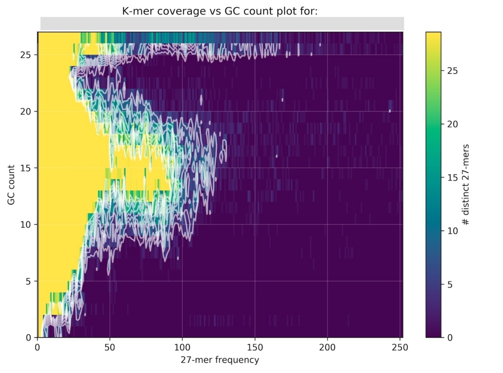
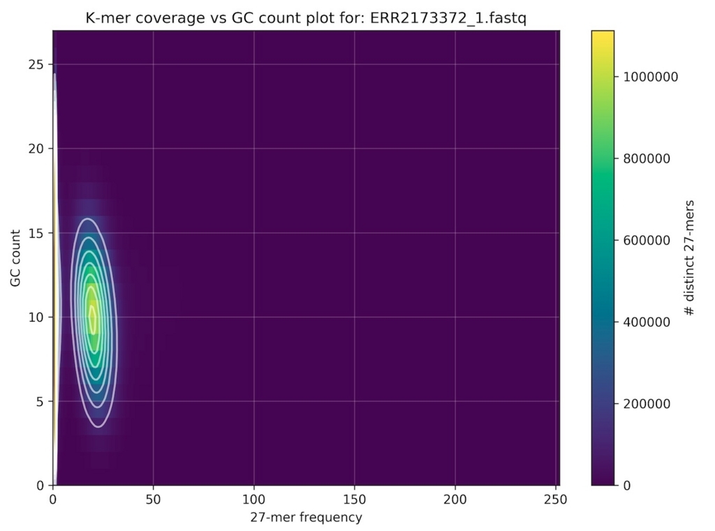
k-merサイズ27でペアエンドのfastqを分析。

kat gcp -t 10 -x 1 -y 10000 -m 27 -o gcc -v sample1_*.fastq

シロイヌナズナのシーケンスデータ分析結果。
f:id:kazumaxneo:20180429205507j:plain

激しくコンタミがある バクテリアのシーケンスデータ分析結果。 

f:id:kazumaxneo:20180501115356j:plain


comp: Compares jellyfish K-mer count hashes.

kat comp

$ kat comp

Kmer Analysis Toolkit (KAT) V2.4.2


Usage: kat comp [options] <input_1> <input_2> [<input_3>]


Compares jellyfish K-mer count hashes.


There are two main use cases for this tool.  The first is to compare K-mers from two K-mer hashes both representing K-mer counts for reads.  The intersected output forms a matrix that can be used to show how related both spectra are via a density plot.  The second use case is to compare K-mers generated from reads to those generated from an assembly, in this case the dataset for the reads must be provided first and the assembly second.  This also produces a matrix containing the intersection of both spectra, but this is instead visualised via a stacked histogram.

There is also a third use case where K-mers from a third dataset as a filter, restricting the analysis to the K-mers present on that set.  The manual contains more details on specific use cases.


Options:

  -o [ --output_prefix ] arg (=kat-comp) Path prefix for files generated by this program.

  -t [ --threads ] arg (=1)              The number of threads to use.

  -x [ --d1_scale ] arg (=1)             Scaling factor for the first dataset - float multiplier

  -y [ --d2_scale ] arg (=1)             Scaling factor for the second dataset - float multiplier

  -i [ --d1_bins ] arg (=1001)           Number of bins for the first dataset.  i.e. number of rows in the matrix

  -j [ --d2_bins ] arg (=1001)           Number of bins for the second dataset.  i.e. number of rows in the matrix

  --d1_5ptrim arg (=0)                   Ignore the first X bases from reads in dataset 1.  If more that one file is provided for dataset 1 you can specify different values 

                                         for each file by seperating with commas.

  --d2_5ptrim arg (=0)                   Ignore the first X bases from reads in dataset 2.  If more that one file is provided for dataset 2 you can specify different values 

                                         for each file by seperating with commas.

  -N [ --non_canonical_1 ]               If counting fast(a/q) for input 1, store explicit kmer as found.  By default, we store 'canonical' k-mers, which means we count both 

                                         strands.

  -O [ --non_canonical_2 ]               If counting fast(a/q) for input 2, store explicit kmer as found.  By default, we store 'canonical' k-mers, which means we count both 

                                         strands.

  -P [ --non_canonical_3 ]               If counting fast(a/q) for input 3, store explicit kmer as found.  By default, we store 'canonical' k-mers, which means we count both 

                                         strands.

  -m [ --mer_len ] arg (=27)             The kmer length to use in the kmer hashes.  Larger values will provide more discriminating power between kmers but at the expense of 

                                         additional memory and lower coverage.

  -H [ --hash_size_1 ] arg (=100000000)  If kmer counting is required for input 1, then use this value as the hash size.  If this hash size is not large enough for your 

                                         dataset then the default behaviour is to double the size of the hash and recount, which will increase runtime and memory usage.

  -I [ --hash_size_2 ] arg (=100000000)  If kmer counting is required for input 2, then use this value as the hash size.  If this hash size is not large enough for your 

                                         dataset then the default behaviour is to double the size of the hash and recount, which will increase runtime and memory usage.

  -J [ --hash_size_3 ] arg (=100000000)  If kmer counting is required for input 3, then use this value as the hash size.  If this hash size is not large enough for your 

                                         dataset then the default behaviour is to double the size of the hash and recount, which will increase runtime and memory usage.

  -d [ --dump_hashes ]                   Dumps any jellyfish hashes to disk that were produced during this run. Normally, this is not recommended, as hashes are slow to load 

                                         and will likely consume a significant amount of disk space.

  -g [ --disable_hash_grow ]             By default jellyfish will double the size of the hash if it gets filled, and then attempt to recount.  Setting this option to true, 

                                         disables automatic hash growing.  If the hash gets filled an error is thrown.  This option is useful if you are working with large 

                                         genomes, or have strict memory limits on your system.

  -n [ --density_plot ]                  Makes a density plot.  By default we create a spectra_cn plot.

  -p [ --output_type ] arg (=png)        The plot file type to create: png, ps, pdf.

  -h [ --output_hists ]                  Whether or not to output histogram data and plots for input 1 and input 2

  -v [ --verbose ]                       Print extra information.

  --help                                 Produce help message.

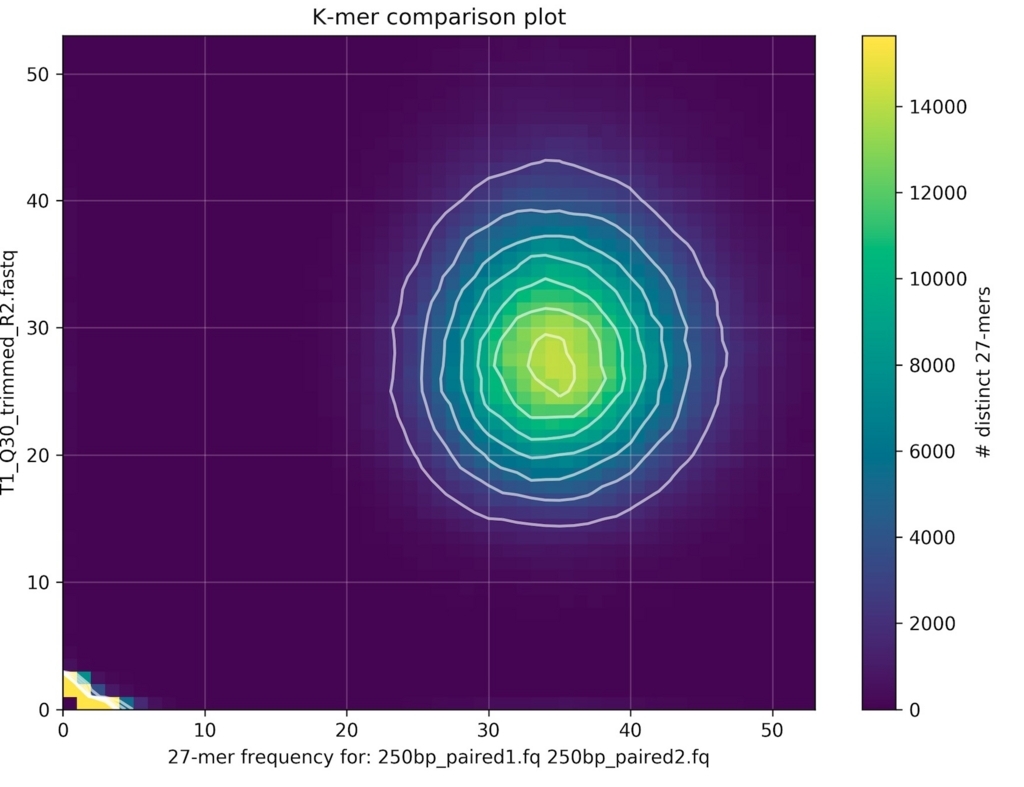
2サンプルのfastqを比較する。 

kat comp -t 10 -v 'sample1_1.fq sample1_2.fq' 'sample2_1.fq sample2_2.fq'

kat-comp-main.mxとヒストグラムが出力される。ここではここでは同じゲノムのリアルデータ(PCR free)とシミュレーションデータを比較した。

f:id:kazumaxneo:20180501133141p:plain

plotコマンドで2サンプルのbiasを分析。density plot出力。

kat plot density kat-comp-main.mx 
f:id:kazumaxneo:20180501133334j:plain

plotコマンドで2サンプルのbiasを分析。ヒストグラム出力。

kat plot spectra-mx -i kat-comp-main.mx 


cold:  Contig Length and Duplication analysis tool.

kat cold

$ kat cold

Kmer Analysis Toolkit (KAT) V2.4.2


Usage: kat cold [options] <assembly> <reads>


COntig Length and Duplication analysis tool


Calculates median read k-mer coverage, assembly k-mer coverage and GC% across each sequence in the provided assembly. Then, assuming plotting is enabled, the results are converted into a scatter plot, where each point is colored according to a similar scheme used in spectra-cn plots, and sized according to its length.  The y-axis representsmedian read K-mer coverage, and x-axis represents GC%.


 The <assembly> should be a fasta file that is NOT gzipped compressed.  The <reads> can be any number of <fasta/q> files, which CAN be gzipped compressed, or a pre-counted hash.


Options:

  -o [ --output_prefix ] arg (="kat-cold") Path prefix for files generated by this program.

  -x [ --gc_bins ] arg (=1001)             Number of bins for the gc data when creating the contamination matrix.

  -y [ --cvg_bins ] arg (=1001)            Number of bins for the cvg data when creating the contamination matrix.

  -t [ --threads ] arg (=1)                The number of threads to use

  --5ptrim arg (=0)                        Ignore the first X bases from reads.  If more that one file is provided you can specify different values for each file by 

                                           seperating with commas.

  -m [ --mer_len ] arg (=27)               The kmer length to use in the kmer hashes.  Larger values will provide more discriminating power between kmers but at the expense 

                                           of additional memory and lower coverage.

  -H [ --hash_size ] arg (=100000000)      If kmer counting is required, then use this value as the hash size for the reads.  We assume the assembly should use half this 

                                           value.  If this hash size is not large enough for your dataset then the default behaviour is to double the size of the hash and 

                                           recount, which will increase runtime and memory usage.

  -d [ --dump_hashes ]                     Dumps any jellyfish hashes to disk that were produced during this run. Normally, this is not recommended, as hashes are slow to 

                                           load and will likely consume a significant amount of disk space.

  -g [ --disable_hash_grow ]               By default jellyfish will double the size of the hash if it gets filled, and then attempt to recount.  Setting this option to true,

                                           disables automatic hash growing.  If the hash gets filled an error is thrown.  This option is useful if you are working with large 

                                           genomes, or have strict memory limits on your system.

  -p [ --output_type ] arg (=png)          The plot file type to create: png, ps, pdf.

  -v [ --verbose ]                         Print extra information.

  --help                                   Produce help message.

アセンブリしたfastaと、アセンブリに使ったfastqを指定する。

kat cold -t 10 -v assembly.fasta sample1_*.fastq

少しだけコンタミがある バクテリアのシーケンスデータと、そのspadesアセンブリFASTAの分析結果。

f:id:kazumaxneo:20180429214407j:plain


filter: K-mer filtering tools。kmerseqがある。

kat filter

$ kat filter

Kmer Analysis Toolkit (KAT) V2.4.2


Usage: kat filter <mode>


Filtering tools


First argument should be the filter mode you wish to use:

  * kmer:            Filters a jellyfish k-mer hash using user defined properties.

  * seq:             Filters sequences in a file based on k-mers in a given hash


Options:

  -v [ --verbose ]      Print extra information

  --help                Produce help message.

はじめにjellyfishなどでk-mer分析を行う。 

jellyfish count -m 27 -s 10000000 -t 10sample1_*fq -o mer_counts.jf

k-mer 頻度10以上1000以下、k-merのGC率50-60%だけ抽出する。

kat filter kmer -t 10 -c 5 -d 1000 -g 50 -h 60 -o filtered mer_counts.jf 


plot: Plotting tools.

kat plot

$ kat plot

Kmer Analysis Toolkit (KAT) V2.4.2


Usage: kat plot <mode>


Create K-mer Plots


First argument should be the plot mode you wish to use:

  * density:         Creates a density plot from a matrix created with the "comp" tool or the

                     "GCP" tool.  Typically this is used to compare two K-mer hashes produced

                     by different NGS reads, or to represent the kmer coverage vs GC count plots.

  * profile:         Creates a K-mer coverage plot for a single sequence.  Takes in fasta

                     coverage output from the "sect" tool

  * spectra-cn:      Creates a stacked histogram using a matrix created with the "comp" tool.

                     Typically this is used to compare a jellyfish hash produced from a read set

                     to a jellyfish hash produced from an assembly. The plot shows the amount of

                     distinct K-mers absent, as well as the copy number variation present within

                     the assembly.

  * spectra-hist:    Creates a K-mer spectra plot for a set of K-mer histograms produced either

                     by jellyfish-histo or kat-histo.

  * spectra-mx:      Creates a K-mer spectra plot for a set of K-mer histograms that are derived

                     from selected rows or columns in a matrix produced by the "comp".

  * cold:            Takes in a stats file produced by "cold" and produces a scatter plot of

                     median read K-mer coverage vs GC% for each contig in the assembly, with

                     point's size being adjusted by sequence length


Options:

  -v [ --verbose ]      Print extra information

  --help                Produce help message.


 plotはcompコマンドでの例のように、他のコマンドと組み合わせて使う。


この他、カバレッジを推定するsectがある。 


KATマニュアルのwalkthroughセクションを読むと、サンブルのバッチエフェクト、シーケンスバイアスの調べ方などを学べます。

http://kat.readthedocs.io/en/latest/walkthrough.html#comparing-r1-v-r2-in-an-illumina-pe-dataset


追記

ゲノムサイズ推定


引用

KAT: a K-mer analysis toolkit to quality control NGS datasets and genome assemblies

Daniel Mapleson, Gonzalo Garcia Accinelli, George Kettleborough, Jonathan Wright, and Bernardo J. Clavijo

Bioinformatics. 2017 Feb 15; 33(4): 574–576.


k-merを使ったリードフィルタリングを行う Cookiecutter

2022/02/08 インストール追記


 次世代シークエンシング技術は、より安価になり、ルーティンの分析に役立っている。アセンブリの前に未処理のリードから特定のシーケンスを抽出または削除することを必要とする多くのタスクがある。抽出された領域特異的なリード(例えば、mtDNAまたはrRNAからの)のほんの一部使えば、得られたアセンブリおよびその分析の速度および品質を有意に改善することができる(Hahn et al、2013)。一方、リードトリミングは常に望ましい戦略ではなく、技術的なシーケンスの断片を含むすべてのリードを削除する方が効果的で簡単である。このような除去手順は、例えば、擬似ゲノム接尾辞配列作成(Kowalski et al、2015)に必要とされるのと同じリード長を維持する。
いくつかのツールは、rawリード処理のために開発された:アダプタ配列のライブラリに基づいたトリミング(Bolger et al、2014; Martin、2011)、カバレッジとアラインメントの同一性(Schmieder and Edwards、2011a) (Morgan et al。、2009)、シーケンスエントロピー尺度(Schmieder and Edwards、2011b)に従ってリードを取り除き、それらのコピー数に従ってリードを取り除く(Brownら、2012)。しかし、任意のシーケンスとの類似性に基づいてリードをフィルタリングするためのツールが不足している。この問題を解決するために、Cookiecutterツールを開発した。
 Cookiecutterは、任意の解析パイプラインに簡単に統合できるスタンドアロンコマンドラインツールパッケージである。 Cookiecutterは、1つまたは複数のFASTQファイルを入力として受け取り、フィルタリングのためにk-mersのリストを含むファイルを必要とする。そのリストは、ユーザーが提供するか、提供されたFASTAファイルのCookiecutterによって生成される。 Cookiecutterは、シングルエンドリードとペアエンドリード両方を処理できる。ペアエンドリードの場合、Cookiecutterは両方のリードがフィルタリングを通過するとペアを維持する。ペアの1つがフィルタリングされた場合、他方のリードはシングルエンドとして別出力される。


インストール

mac os10.13でテストした。

依存

Github

リリースから実行ファイルのBinaryがダウンロードできる。

https://github.com/ad3002/Cookiecutter/releases

wget  https://github.com/ad3002/Cookiecutter/releases/download/v1.0.0/cookiecutter_osx.tar.gz
tar -xvzf cookiecutter_osx.tar.gz
cd cookiecutter_osx.65cwMW/bin/
export PATH=$PWD:$PATH

#2022/02/08 python2.7の環境を作っていれる
mamba create -n cookiecutter python=2.7 -y
conda activate cookiecutter
wget https://github.com/ad3002/Cookiecutter/releases/download/v1.0.0/cookiecutter_linux_x64.tar.gz
tar -xvzf cookiecutter_linux_x64.tar.gz
cd cookiecutter_linux_x64/bin/
export PATH=$PWD:$PATH

./cookiecutter -h

$ ./cookiecutter -h

usage: cookiecutter [-h] [-v] [-e]

                    {extract,remove,rm_reads,separate,make_library} ...


Cookiecutter: a kmer-based read filtration and extraction tool.


positional arguments:

  {extract,remove,rm_reads,separate,make_library}

    extract             extract reads matching the specified k-mers

    remove              remove reads matching the specified k-mers

    rm_reads            classify reads applying the specified filters

    separate            separate reads matching or unmatching the specified

                        k-mers

    make_library        create a file of k-mers from sequences of the

                        specified FASTA file


optional arguments:

  -h, --help            show this help message and exit

  -v, --version         show program's version number and exit

  -e, --echo            print commands to be launched instead of launching

                        them

cookiecutter make_library -h

$ cookiecutter make_library -h

usage: cookiecutter make_library [-h] -i INPUT [INPUT ...] -o OUTPUT -l LENGTH


Create a library of k-mers from the specified FASTA file.


optional arguments:

  -h, --help            show this help message and exit


required_arguments:

  -i INPUT [INPUT ...], --input INPUT [INPUT ...]

                        a list of FASTA files

  -o OUTPUT, --output OUTPUT

                        an output file of k-mers

  -l LENGTH, --length LENGTH

                        the length of generated k-mers

cookiecutter remove -h

$ cookiecutter remove -h

usage: cookiecutter remove [-h]

                           (-i INPUT [INPUT ...] | -1 FASTQ1 [FASTQ1 ...])

                           [-2 FASTQ2 [FASTQ2 ...]] [-t THREADS] -f FRAGMENTS

                           -o OUTPUT


Removes reads according to a given list of k-mers and outputs only reads

without any matches to the provided k-mer list.


optional arguments:

  -h, --help            show this help message and exit

  -2 FASTQ2 [FASTQ2 ...], --fastq2 FASTQ2 [FASTQ2 ...]

                        a FASTQ file of the second paired-end reads

  -t THREADS, --threads THREADS

                        the number of threads for parallel processing of

                        multiple input files (default: 1)


required arguments:

  -i INPUT [INPUT ...], --input INPUT [INPUT ...]

                        a FASTQ file of single-end reads

  -1 FASTQ1 [FASTQ1 ...], --fastq1 FASTQ1 [FASTQ1 ...]

                        a FASTQ file of the first paired-end reads

  -f FRAGMENTS, --fragments FRAGMENTS

                        a file of k-mers

  -o OUTPUT, --output OUTPUT

                        a directory for output files

uesaka-no-Air-2:bin kazumaxneo$ 

cookiecutter extract -h

$ cookiecutter extract -h

usage: cookiecutter extract [-h]

                            (-i INPUT [INPUT ...] | -1 FASTQ1 [FASTQ1 ...])

                            [-2 FASTQ2 [FASTQ2 ...]] [-t THREADS] -f FRAGMENTS

                            -o OUTPUT


Extracts reads according to a given list of k-mers and outputs only the reads

that matched the list.


optional arguments:

  -h, --help            show this help message and exit

  -2 FASTQ2 [FASTQ2 ...], --fastq2 FASTQ2 [FASTQ2 ...]

                        a FASTQ file of the second paired-end reads

  -t THREADS, --threads THREADS

                        the number of threads for parallel processing of

                        multiple input files (default: 1)


required arguments:

  -i INPUT [INPUT ...], --input INPUT [INPUT ...]

                        a FASTQ file of single-end reads

  -1 FASTQ1 [FASTQ1 ...], --fastq1 FASTQ1 [FASTQ1 ...]

                        a FASTQ file of the first paired-end reads

  -f FRAGMENTS, --fragments FRAGMENTS

                        a file of k-mers

  -o OUTPUT, --output OUTPUT

                        a directory for output files

cookiecutter separate -h

$ cookiecutter separate -h

usage: cookiecutter separate [-h]

                             (-i INPUT [INPUT ...] | -1 FASTQ1 [FASTQ1 ...])

                             [-2 FASTQ2 [FASTQ2 ...]] [-t THREADS] -f

                             FRAGMENTS -o OUTPUT


Outputs both matched and not matched reads in separate files.


optional arguments:

  -h, --help            show this help message and exit

  -2 FASTQ2 [FASTQ2 ...], --fastq2 FASTQ2 [FASTQ2 ...]

                        a FASTQ file of the second paired-end reads

  -t THREADS, --threads THREADS

                        the number of threads for parallel processing of

                        multiple input files (default: 1)


required arguments:

  -i INPUT [INPUT ...], --input INPUT [INPUT ...]

                        a FASTQ file of single-end reads

  -1 FASTQ1 [FASTQ1 ...], --fastq1 FASTQ1 [FASTQ1 ...]

                        a FASTQ file of the first paired-end reads

  -f FRAGMENTS, --fragments FRAGMENTS

                        a file of k-mers

  -o OUTPUT, --output OUTPUT

                        a directory for output files

cookiecutter rm_reads -h

$ cookiecutter rm_reads -h

usage: cookiecutter rm_reads [-h]

                             (-i INPUT [INPUT ...] | -1 FASTQ1 [FASTQ1 ...])

                             [-2 FASTQ2 [FASTQ2 ...]] [-t THREADS] [-p POLYGC]

                             [-l LENGTH] [-d] [-c DUST_CUTOFF] [-k DUST_K]

                             [-N] -f FRAGMENTS -o OUTPUT


The rm_reads tool is an extended version of remove enhanced with the DUST

filter, removing reads containing (G)n- and (C)n-tracks and unknown

nucleotides and filtering reads by their length; also its output includes both

filtered and unfiltered reads.


optional arguments:

  -h, --help            show this help message and exit

  -2 FASTQ2 [FASTQ2 ...], --fastq2 FASTQ2 [FASTQ2 ...]

                        a FASTQ file of the second paired-end reads

  -t THREADS, --threads THREADS

                        the number of threads for parallel processing of

                        multiple input files (default: 1)

  -p POLYGC, --polygc POLYGC

                        the polyG/polyC sequence length cutoff (default: 13)

  -l LENGTH, --length LENGTH

                        the read length cutoff (default: 50)

  -d, --dust            use the DUST filter (default: False)

  -c DUST_CUTOFF, --dust_cutoff DUST_CUTOFF

                        the score cutoff for the DUST filter (default: 2)

  -k DUST_K, --dust_k DUST_K

                        the window size for the DUST filter (default: 4)

  -N, --filterN         filter reads by the presence of Ns (default: False)


required arguments:

  -i INPUT [INPUT ...], --input INPUT [INPUT ...]

                        a FASTQ file of single-end reads

  -1 FASTQ1 [FASTQ1 ...], --fastq1 FASTQ1 [FASTQ1 ...]

                        a FASTQ file of the first paired-end reads

  -f FRAGMENTS, --fragments FRAGMENTS

                        a file of k-mers

  -o OUTPUT, --output OUTPUT

                        a directory for output files


ラン

make_library

はじめにk-merライブラリを作る必要がある。ゲノム配列を指定する。k-merサイズは27とする。

cookiecutter make_library -i ref.fa -o adapters.txt -l 27 

 > head adapters.txt

$ head adapters.txt 

TTGATCCCTCTTCATATCTAGGAGTTT 1

CTCCCTGGCCCTGGGGGGTCAGTTGCT 1

GGCCAGGGCTTCGCTATACAGACCAGA 1

AAACCCAAACAGCTTCGGCAGGATTGT 1

ATAATCAGTTTTAATAAAGCCGAACTC 1

ATAAGCCGGCACCCGGAAAGGAAACTC 1

ATCGCCTGGGCCGACGGGGCACGGTGG 1

TAACCGGGCGGAAACTAAATATTTACC 1

ATGGCCTGCACTTGATGCAAAAACCAA 1

AGAGAACACCAAGAAAATACCCATAGT 1

大きなゲノムやfastqの分析には時間がかかるので、コンパチブルのJellyfish2を使う。

jellyfish count -m 27 -s 10G -t 8 --text -o kmer_library.dat input.fastq 


remove  searches given k-mers in reads and outputs the reads without any matches to the k-mers;

上記ゲノムのk-merを含むリードを除く。adapters.txtとfastqファイルを指定する。

cookiecutter remove -i input.fq -f adapters.txt -o filtered

 filteredディレクトリにマッチしなかったリードのfastqが出力される。ペアエンドリードは"-i"の代わりに-1"と"-2"を使う。


extract searches given k-mers in reads and outputs the reads that matched the k-mers;

cookiecutter extract -i input.fq -f adapters.txt -o filtered

 extractだとマッチしたリードが出力される。


separate searches given k-mers in reads and outputs both matched and unmatched reads to two separate files. 

cookiecutter separate -1 pair1.fq -2 pair2.fq -f adapters.txt -o output_dir

separateだとマッチしたリードとマッチしなかったリードが別ファイルに分けられて両方出力される。


より複雑なフィルタリングを行うにはrm_readsコマンドを使う。長さ、low complexility、poly GC、NNN、などのフィルタリングができる。

rm_reads is an extension of remove that additionally provides options to filter reads by the presence of (C)n/(G)n tracks or unknown nucleotides, read length or low sequence complexity and outputs both filtered and unfiltered reads;

cookiecutter rm_reads -1 pair1.fq -2 pair2.fq -f adapters.txt -o output_dir --polygc 13 --length 50 --dust --filterN

 テストした時は-Nフィルタだけ機能しなかった。


メモリ使用量が多いのと計算負荷が高いのが気になりますが、上手く使えば、コンタミを除いたり、メタゲノムからターゲットゲノムを濃縮したり、様々な用途に活用できると思います。 複数ファイルも指定できます。GithubのREADMEを参照してください。


BBtoolsのBBDukもk-merフィルタリングが可能です。


引用

Cookiecutter: a tool for kmer-based read filtering and extraction

Ekaterina Starostina, Gaik Tamazian, Pavel Dobrynin, Stephen O'Brien, Aleksey Komissarov

bioRxiv preprint first posted online Aug. 16, 2015; doi: http://dx.doi.org/10.1101/024679.


ロングリードのクオリティ分析とトリミングを行う Filtlong

#2022/04/20 追記


 FiltlongはONTのロングリードのクオリティ分析やクオリティ、リード長のトリミングが行えるツール。ウルトラロングリードを低クオリティ領域でカットして、分割出力する機能も備える。2018年4月現在Githubで公開されている。


インストール

mac os10.13に導入した。

依存

Github

https://github.com/rrwick/Filtlong

#conda
mamba install -c bioconda filtlong -y

git clone https://github.com/rrwick/Filtlong.git
cd Filtlong
make -j 4
bin/filtlong -h

usage: filtlong {OPTIONS} [input_reads]


Filtlong: a quality filtering tool for Nanopore and PacBio reads


positional arguments:

    input_reads                         input long reads to be filtered


optional arguments:

    output thresholds:

        -t[int], --target_bases [int]       keep only the best reads up to this many total bases

        -p[float], --keep_percent [float]   keep only this percentage of the best reads (measured by bases)

        --min_length [int]                  minimum length threshold

        --max_length [int]                  maximum length threshold

        --min_mean_q [float]                minimum mean quality threshold

        --min_window_q [float]              minimum window quality threshold


    external references (if provided, read quality will be determined using these instead of from the Phred scores):

        -a[file], --assembly [file]         reference assembly in FASTA format

        -1[file], --illumina_1 [file]       reference Illumina reads in FASTQ format

        -2[file], --illumina_2 [file]       reference Illumina reads in FASTQ format


    score weights (control the relative contribution of each score to the final read score):

        --length_weight [float]             weight given to the length score (default: 1)

        --mean_q_weight [float]             weight given to the mean quality score (default: 1)

        --window_q_weight [float]           weight given to the window quality score (default: 1)


    read manipulation:

        --trim                              trim non-k-mer-matching bases from start/end of reads

        --split [split]                     split reads at this many (or more) consecutive non-k-mer-matching bases


    other:

        --window_size [int]                 size of sliding window used when measuring window quality (default: 250)

        --verbose                           verbose output to stderr with info for each read

        --version                           display the program version and quit


    -h, --help                          display this help menu


For more information, go to: https://github.com/rrwick/Filtlong


ラン

リファレンスがない時のクオリティ分析。

filtlong --min_length 1000 --keep_percent 90 \
--target_bases 500000000 input.fastq.gz | \
gzip - > output.fastq.gz
  • --min_length 1000   Discard any read which is shorter than 1 kbp.
  • --keep_percent 90   Throw out the worst 10% of reads. This is measured by bp, not by read count. So this option throws out the worst 10% of read bases.
  • --target_bases 500000000   Remove the worst reads until only 500 Mbp remain, useful for very large read sets. If the input read set is less than 500 Mbp, this setting will have no effect.
  • input.fastq.gz   The input long reads to be filtered (must be FASTQ format).


リファレンスとなるハイクオリティなショートリードがある時のクオリティ分析。このモードではロングリードのquality scoreは使わずショートリードとk-merマッチを行う。ONTのロングリードのクオリティスコアを使わないことで分析精度が上がるとされる。

filtlong -1 illumina_1.fastq.gz -2 illumina_2.fastq.gz \ 
--min_length 1000 --keep_percent 90 --target_bases 500000000 \
--trim --split 500 input.fastq.gz | gzip > output.fastq.gz
  •  -1 illumina_1.fastq.gz -2 illumina_2.fastq.gz   Use Illumina reads as an external reference. You can instead use "-a" to provide an assembly as a reference, but Illumina reads are preferable if available.


クオリティ分析とトリミングおよびウルトラロングリードのsplit triminng。

filtlong -1 illumina_1.fastq.gz -2 illumina_2.fastq.gz --min_length 1000 \
--keep_percent 90 --target_bases 500000000 --trim --split 500 \
input.fastq.gz | gzip > output.fastq.gz
  • --trim   Trim bases from the start and end of reads which do not match a k-mer in the reference. This ensures the each read starts and ends with good sequence.
  • --split 500   Split reads whenever 500 consequence bases fail to match a k-mer in the reference. This serves to remove very poor parts of reads while keeping the good parts. A lower value will split more aggressively and a higher value will be more conservative.

split機能(--split)によりウルトラロングリードのpoor qualityな領域でリードが切断され、500bp以上の領域が確保できれば別リードとして出力される。

f:id:kazumaxneo:20180430205752j:plain

公式より


リード長優先トリミング

filtlong -1 illumina_1.fastq.gz -2 illumina_2.fastq.gz --min_length 1000\
--keep_percent 90 --target_bases 500000000 --trim --split 1000 --length_weight 10 \
input.fastq.gz | gzip > output.fastq.gz
  • --length_weight 10   A length weight of 10 (instead of the default of 1) makes read length more important when choosing the best reads.
  • --split 1000   This larger split value makes Filtlong less likely to split a read. I.e. a read has to have a lot of consecutive bad bases before it gets split. This helps to keep the output reads longer.


クオリティ優先トリミング

filtlong -1 illumina_1.fastq.gz -2 illumina_2.fastq.gz --min_length 1000 \ 
--keep_percent 90 --target_bases 500000000 --trim --split 100 --mean_q_weight 10 \
input.fastq.gz | gzip > output.fastq.gz
  •  --mean_q_weight 10   A mean quality weight of 10 (instead of the default of 1) makes mean read quality more important when choosing the best reads.
  • --split 100   This smaller split value makes Filtlong split reads more often. I.e. even a relatively small stretch of bad bases will result in a split, giving shorter reads but of higher quality.


Githubの公開ページでは、バクテリアのmultiplex minion sequenceのデータを使った例が示されています。

引用

https://github.com/rrwick/Filtlong


k-mersからゲノムの類似性を高速計算する kWIP


 DNAシークエンシングの主な用途は、試料の遺伝的構成を互いに比較して共通性を同定し、したがって関連性を検出するか、またはその差を利用して機能を解明することである。最初に、仮定された遺伝的系統および複製を確認するか、またはサンプルを家族、集団および種にグループ化することを試みる。幅広いサンプルのコレクション間の遺伝的関連性を推定するには、バイアスを避け、サンプルあたりのコストを最小限に抑える必要がある。

 今日、集団ゲノミクスの研究の大部分は、NGSを用いて行われている[論文より ref.1]。全ゲノムシーケンスデータを分析するために一般的に用いられる方法は2つの補間する方法に基づいている。すなわちリファレンスとするゲノムをアセンブリし、リシーケンスしたサンプルをこのゲノムにマッピングしてバリアントをコールする。このアプローチは、モデル生物においては機能的であるが、理想的な方法ではない。リファレンスとなる個体の選択は大部分がランダムであるため、リファレンスゲノムのアセンブリには時間とコストがかかるし[ref.2,3]、不適切なリファレンスゲノム配列に基づく分析は、リファレンスと異なっているか欠けている場合などバイアスを受けやすい[ref.4,5]。遺伝的関連性を測定するアラインメントフリーの方法は、このリファレンスゲノムバイアスを克服するのに役立つ。 

 懸念事項のもう一つは、サンプルの識別となる。最近のレビュー[ref.6]は、誤った標本化が驚くべき速度で起こっていることを発見した(pubmed)。集団遺伝子プロジェクトにおけるサンプル数の増加に伴い、正確かつ一貫したメタデータの問題は、技術的(mix-up)と生物学的(misidentification)といういくつかのレベルで発生する。大規模なフィールド、および遺伝子バンクコレクション全体がDNAシーケンス解析されている。ラボから実験室までのサンプル処理では、シーケンスリードファイルや最終的なデータ・リポジトリへのアップロードまで、サンプルとファイルが混在して誤って表示される可能性が十分にある。この問題は、そのような取り組みのしばしば非常に協力的な性質によってしばしば悪化する。しかしながら、いくつかの誤った同定は、(compilo)種複合体における倍数性、潜在性の種、またはサブのゲノムレベルの変化など、分子遺伝学的分析がなければ事実上検出されない可能性がある[ref.7]。残念なことに、この隠された変異の多くは、ショートリードシーケンシングデータからゲノム全体の遺伝的関連性を計算するための前述の現在のベストプラクティスに従うことによって容易に見過ごされる。誤ったサンプル同定および発散レベルの過小評価は、GWASに使用するサンプルおよび集団、欠落している遺伝性は実際にはメタデータ内に存在する可能性がある。

 アライメントフリー配列比較は、配列アライメントのプロセスを回避することにより、これらの困難に対処することを目的とする(一部略)。いくつかのアライメントフリー配列比較ツールは、依然として基礎となるゲノム配列の事前知識を必要とするため、デノボツールとしてのそれらの使用が妨げられる。最近、デノボ比較を可能にするいくつかのアルゴリズムが公開されている。これらのエクステンションは全てシーケンシング・リードからの系統発生的関係を再構築しようと試みる。 Spaced [ref.13,16]は、系統学的再構成の性能を向上させるために、間隔の取られたシード(小さなk-mersを互いから、または点在する無視された塩基と短い距離)でJensen-Shannon distanceを用いる。 Cnidaria [ref.17]とAAF [ref.18]はJaccard距離を用いて系統を再構築するが、mash [ref.19]はJaccard距離のMinHash近似を用いて同じ効果を得る。

 最も確立され、研究されたアライメントフリーの配列比較測定基準の1つは、D2統計である[ref.8,10]。これは、k-merマッチの数によって2つの配列間の差異を測定する。まず、全てのk量体を各配列中で計数し、計数ベクターに記録する。次に、これらのベクトルの差を測定する。元のD2統計量の場合、これは単にベクトル積を構築することによって達成される。観測されたk-merスペクトラウムをモデル化し相関させることによって精度を改善することを目的としたD2統計量のいくつかの派生、例えばD*2、Ds2が長年にわたって開発されている[ref.8,20-23]。これらの統計は次世代シークエンスデータ[ref.24]に拡張され、メタゲノム比較[ref.25]にうまく適用されたが、D2やDS2のようなD2統計的導関数は計算速度が遅く、定義が難しい。

 ここでは、k-merベースの配列比較に2つの概念を導入して組み合わせる遺伝的関連性を推定するための新しい指標であるk-mer Weighted Inner Productを提示する。 D2統計量と同様に、類似性測度はk-mer数の内積であるが、まず、各k-merを比較するのではなく、むしろすべてのk-mersを確率データ構造にハッシュする:Sketch[ref.26]。得られたSketchは、事実上、k-merカウントのベクトルである。重要なことに、すべてのサンプルのSketchは一定のサイズを持つ。第2に、情報理論上の重みづけを導入して、関連する遺伝子信号をノイズよりも高くする。次に、集団全体の頻度から導出された情報量によって重み付けされた、k-merカウント間の内積によって対の類似性が計算される。この手順は、シーケンシングリードから直接、メトリックであるk-mer加重内積を計算するソフトウェアツール(kWIP)で実装されている。著者らはシミュレーションと、公開されたデータセットの再分析によって、kWIPがサンプル間の遺伝的関連性を素早く正確に検出できることを示す。


マニュアル

https://kwip.readthedocs.io/en/latest/


インストール

ubuntu14.04に導入した。

Github

##依存
sudo apt-get install zlib1g-dev cmake build-essential git

git clone https://github.com/kdmurray91/kWIP.git
cd kWIP

mkdir build && cd build
cmake .. -DCMAKE_INSTALL_PREFIX=${HOME}
make
make test
make install
cd bin/
./kwip

> ./kwip 

$ ./kwip

kwip version 0.2.0-13-g3cf8a9e


USAGE: ./kwip [options] hashes


OPTIONS:

-t, --threads Number of threads to utilise. [default N_CPUS]

-k, --kernel Output file for the kernel matrix. [default None]

-d, --distance Output file for the distance matrix. [default stdout]

-U, --unweighted Use the unweighted inner proudct kernel. [default off]

-w, --weights Bin weight vector file (input, or output w/ -C).

-C, --calc-weights Calculate only the bin weight vector, not kernel matrix.

-h, --help Print this help message.

-V, --version Print the version string.

-v, --verbose Increase verbosity. May or may not acutally do anything.

-q, --quiet Execute silently but for errors.


Each sample's oxli Countgraph should be specified after arguments:

./kwip [options] sample1.ct sample2.ct ... sampleN.ct

ビルド済みのバイナリもダウンロードできる。

https://kwip.readthedocs.io/en/latest/installation.html 


ラン

rice 3000 genome project (pubmed) のシーケンスを使用して、流れを確認する(リンク)。 


ワーキングディレクトリの作成

mkdir ~/rice_kwip 
cd ~/rice_kwip


公式ではvirtualenvwrapperでpythonの固有環境を作って作業しているが、ここでは使わない。

pip install srapy 
pip install khmer


ヒアドキュメントでダウンロードリストファイルを作成。いずれもシングルエンドのシーケンスデータ。

cat >sra_run_ids.txt <<EOF 
ERR626208
ERR626209
ERR626210
ERR626211
ERR619511
ERR619512
ERR619513
ERR619514
EOF


 シーケンスデータダウンロードディレクトリを作成し、SRApy(リンク)でダウンロードを実行。合計4.3GBある。

mkdir sra_files
get-run.py -s -f sra_run_ids.txt -d sra_files/

追記)sra-toolikitを使ってもダウンロードできる。asperaを使うなら"-a"オプションでascpの実行ファイルパスと作成した秘密鍵の場所を指定する。

prefetch --option-file sra_run_ids.txt --max-size 1000000000

#終わったらsra_files/に移動
mv ~/ncbi/public/sra/ERR626* sra_files/


 fastqへの変換。fastq-dumpコマンドがないならbrew  install sratoolkitでSRA toolkitを導入する。出力はgz圧縮する。forで回して一括変換する。

mkdir fastqs
for srr in $(cat sra_run_ids.txt)
do
fastq-dump \
--split-spot \
--skip-technical \
--stdout \
--readids \
--defline-seq '@$sn/$ri' \
--defline-qual '+' \
sra_files/${srr}.sra | \
gzip -1 > fastqs/${srr}.fastq.gz
done

fastq/に抽出されたfq.gzが保存される。


hash計算ディレクトリを作成し、khmerのload-into-counting.pyで

mkdir hashes
for srr in $(cat sra_run_ids.txt)
do
load-into-counting.py \
-N 1 \
-x 1e9 \
-k 20 \
-b \
-f \
-s tsv \
hashes/${srr}.ct.gz \
fastqs/${srr}.fastq.gz
done


全hashファイルを指定してkwip実行。

kwip -v -t 2 -k rice.kern -d rice.dist hashes/*.ct.gz 

  kernel matrixファイルとdistance matrixファイルが出力される。

> cat kernel matrix

$ cat rice.kern

ERR619511 ERR619512 ERR619513 ERR619514 ERR626208 ERR626209 ERR626210 ERR626211

ERR619511 6.11354e+08 3.61427e+08 3.69794e+08 3.54549e+08 1.79463e+08 1.78418e+08 1.86159e+08 1.7704e+08

ERR619512 3.61427e+08 5.58085e+08 3.51861e+08 3.3726e+08 1.67822e+08 1.67005e+08 1.74017e+08 1.65437e+08

ERR619513 3.69794e+08 3.51861e+08 5.79062e+08 3.45128e+08 1.72347e+08 1.7169e+08 1.78807e+08 1.70043e+08

ERR619514 3.54549e+08 3.3726e+08 3.45128e+08 5.41048e+08 1.63905e+08 1.63253e+08 1.70158e+08 1.61586e+08

ERR626208 1.79463e+08 1.67822e+08 1.72347e+08 1.63905e+08 4.81631e+08 2.83639e+08 2.94275e+08 2.81749e+08

ERR626209 1.78418e+08 1.67005e+08 1.7169e+08 1.63253e+08 2.83639e+08 4.78399e+08 2.94243e+08 2.80658e+08

ERR626210 1.86159e+08 1.74017e+08 1.78807e+08 1.70158e+08 2.94275e+08 2.94243e+08 5.08735e+08 2.91097e+08

ERR626211 1.7704e+08 1.65437e+08 1.70043e+08 1.61586e+08 2.81749e+08 2.80658e+08 2.91097e+08 4.73382e+08

cat rice.dist 

$ cat rice.dist 

ERR619511 ERR619512 ERR619513 ERR619514 ERR626208 ERR626209 ERR626210 ERR626211

ERR619511 0 0.873197 0.870041 0.87582 1.15695 1.15766 1.15429 1.15837

ERR619512 0.873197 0 0.872979 0.87891 1.16301 1.16344 1.16053 1.16459

ERR619513 0.870041 0.872979 0 0.875678 1.16073 1.16086 1.15807 1.16208

ERR619514 0.87582 0.87891 0.875678 0 1.16526 1.16543 1.16247 1.1668

ERR626208 1.15695 1.16301 1.16073 1.16526 0 0.904545 0.900558 0.905468

ERR626209 1.15766 1.16344 1.16086 1.16543 0.904545 0 0.8984 0.905801

ERR626210 1.15429 1.16053 1.15807 1.16247 0.900558 0.8984 0 0.902021

ERR626211 1.15837 1.16459 1.16208 1.1668 0.905468 0.905801 0.902021 0


distance matrixが得られたので、最後に図で出力する。

Rのfieldsパッケージも使うので、なければCRANからインストールする。

(R内で "install.packages("fields", dependencies = TRUE"

img.Rをカレントにコピーする
cp kWIP/utils/img.R .

#描画してPDF保存
Rscript img.R rice


f:id:kazumaxneo:20180429153720j:plain

f:id:kazumaxneo:20180429153721j:plain

f:id:kazumaxneo:20180429153722j:plain

f:id:kazumaxneo:20180429153725j:plain


f:id:kazumaxneo:20180429153730j:plain

MDS

f:id:kazumaxneo:20180429153735j:plain

2つのグループに分けられた。 


引用

kWIP: The k-mer weighted inner product, a de novo estimator of genetic similarity

Kevin D. Murray, Christfried Webers, Cheng Soon Ong, Justin Borevitz, Norman Warthmann.

PLoS Comput Biol. 2017 Sep; 13(9)


シーケンスデータからk-merスペクトラム分析を行う GenomeScope

 2019 3/5 インストール追記、コマンドのわかりにくい部分を修正

2019 5/14 リンク追加

2019 5/27 docker追加、オプションヘルプ追加

2019 8/27 twitter追記


 ハイスループットシーケンシングにより、新規ゲノムのシーケンシングが日常的に可能になっている。しかしながら、これらのゲノムの最も基本的な特徴、例えばサイズまたはヘテロ接合率などは、最初は未知であり、例えばリードマッパー、デノボアセンブラ、SNPコーラーなどについて適切な分析方法を選択することが困難である(論文より Smolka et al、2015)。これらの特性をあらかじめ決定すれば、変異の数を過小報告したり、ゲノムのかなりの部分をアセンブルできないなど、解析方法がゲノムの複雑性を捕捉をできていないかどうかを明らかにすることができる。これらの特性のいくつかを測定する実験が利用可能であるが、かなりの費用と労力を必要とする可能性がある。

 アセンブルされていないシークエンシングリードからゲノムサイズを推定するための計算手法は現在ほとんどない(Chikhi and Medvedev、2014; Melsted and Halldorsson、2014)。いくつかのゲノムアセンブラアルゴリズムを導くために関連統計を内部的に計算する(Bankevich et al、2012; Gnerre et al、2011)。これらの方法は、BACの長さをライブラリのショットガンサンガーシークエンシングから推測する以前の研究に従っている(Li and Waterman、2003)。しかしながら、ヘテロ接合性の割合などのより複雑な特性を測定するための方法はごくわずかしかなく、これらの方法は使用または解釈が難しい場合がある。 Simpson(2014)は、デノボアセンブリ技術を用いてシーケンシングリードからこれらの特性のいくつかを推定するための計算方法を提案した。しかしながら、この方法は計算集約的であり、より直接的なヘテロ接合率ではなく、変異誘発分枝率のような結果がアセンブリグラフに関連して報告されるので、解釈が難しい場合がある。 GCE法(Liu et al、2013)もまた、ゲノムサイズおよびヘテロ接合率を決定しようと試みるが、完全に自動化されておらず、ユーザがいくつかのカットオフを手動で指定する必要がある。また、実際のシークエンシングデータで推定値が低くなる可能性のあるポアソンカバレッジモデルを使用し、ヘテロ接合性モデルは反復配列のないゲノムに限定されている。

 ここでは、ゲノム特性(全ゲノム長と一倍体ゲノム長、リピート含量とヘテロ接合率のパーセンテージ)、raw シーケンシングデータから全体的なリード特性(カバレッジ、重複とエラー率)を参照ゲノムを必要とせず、k-merプロフィールの統計的分析によって自動的に推測するGenomeScopeを紹介する。 k-merプロファイル(k-merスペクトラムとも呼ばれる)は、k-mers; 長さkの部分文字列がシーケンスリードでどのくらいの頻度で発生するかを測定するもので(一部略)、プロファイルはゲノムの複雑さを反映している:ホモ接合ゲノムは単純なポアソンプロファイルを有するが、ヘテロ接合型ゲノムは特徴的な二峰性のプロファイルを有する(Kajitani et al、2014)。反復はさらに高いk-merスペクトラムでピークを追加するが、シークエンシングエラーとリードのduplicationは低いスペクトラムのfalse k-merと分散の増加を伴いプロファイルを歪ませる(Kelley et al、2010; Miller et al、2011)。

 これらの潜在的複雑さを認識して、本ツールは、ヘテロ接合およびホモ接合、ユニークおよび2コピーの配列の相対存在量を測定するために、k-merプロファイルに4つの等間隔の負の二項分布の混合モデルを適合させる(論文 supplementary S2)。 ポアソン分布に比べて実際のシークエンシングデータはより分散していることが多いため、GenomeScopeはポアソン分布より負の二項分布の混合モデルを使用する(Miller et al、2011)。フィッティングは、Rのnls関数によって実装された非線形最小二乗推定値を使用して計算される(Bates and Watts、1988)。モデルフィッティングをより強固にするために、ゲノムスコープは、シークエンシングエラーによって引き起こされる可能性のある低頻度k-merの異なる部分を除いて、数回のモデルフィッティングを試み、正しいヘテロ接合性およびホモ接合性ピークを決定する際のあいまいさを調整する。パラメータの最終セットは、観察されたk-merプロファイルに対するモデルの残差平方和誤差(RSSE)を最小にするパラメータとして選択される。その後、シーケンスエラーおよびより高いコピー反復は、モデル範囲外のk-mersによって同定され、ホモ接合配列の平均カバレッジ値に対して観察されたk-mer頻度を正規化することによって、全ゲノムサイズを推定する。

GenomeScopeは、コマンドラインのRアプリケーションとしても、また使いやすいWebアプリケーションとしても利用できる。GenomeScopeのコマンドラインまたはオンラインバージョンは、一般的に1分未満で完了し、必要なメモリ量は少なく、推定ゲノム特性を持つテキストファイルも出力する。モデルが収束しない場合、通常、カバレッジが低いか、低品質なため、モデルパラメータを表示せずにk-merプロファイルをプロットし、ユーザが原因を調べることができる。


インストール

ubuntu16.04でテストした。

依存

#ubuntuならapt-getで1.1を導入できる
apt update && apt install -y jellyfish

 本体  Github

git clone https://github.com/schatzlab/genomescope.git
cd genomescope/

Rscript genomescope.R 

$ Rscript genomescope.R -h

USAGE: genomescope.R histogram_file k-mer_length read_length output_dir [kmer_max] [verbose]

> jellyfish count -h

$ jellyfish count -h

Usage: jellyfish count [options] file:path+


Count k-mers or qmers in fasta or fastq files


Options (default value in (), *required):

 -m, --mer-len=uint32                    *Length of mer

 -s, --size=uint64                       *Hash size

 -t, --threads=uint32                     Number of threads (1)

 -o, --output=string                      Output prefix (mer_counts)

 -c, --counter-len=Length in bits         Length of counting field (7)

     --out-counter-len=Length in bytes    Length of counter field in output (4)

 -C, --both-strands                       Count both strand, canonical representation (false)

 -p, --reprobes=uint32                    Maximum number of reprobes (62)

 -r, --raw                                Write raw database (false)

 -q, --quake                              Quake compatibility mode (false)

     --quality-start=uint32               Starting ASCII for quality values (64)

     --min-quality=uint32                 Minimum quality. A base with lesser quality becomes an N (0)

 -L, --lower-count=uint64                 Don't output k-mer with count < lower-count

 -U, --upper-count=uint64                 Don't output k-mer with count > upper-count

     --invalid-char=warn|ignore|error     How to treat invalid characters. The char is changed to a N. (warn)

     --matrix=Matrix file                 Hash function binary matrix

     --timing=Timing file                 Print timing information

     --stats=Stats file                   Print stats

     --usage                              Usage

 -h, --help                               This message

     --full-help                          Detailed help

 -V, --version                            Version

dockerイメージ 

https://hub.docker.com/r/greatfireball/ime_genomescope


ラン

まずfastqファイルを分析する。

jellyfish count -C -m 21 -s 1000000000 -t 12 *fq -o reads.jf
  • -m Length of mer
  • -s Initial hash size
  • -t Number of threads (1)


ヒストグラムファイルを出力する。

jellyfish histo -t 12 reads.jf* > reads.histogram

k-merスペクトラムのグラフを出力する。k-mer_maxの推奨値は1000になっている。

cd genomescope/
Rscript genomescope.R reads.histogram 21 301 output_dir

出力

f:id:kazumaxneo:20190305133520j:plain

cat outdir/summary.txt

GenomeScope version 1.0

k = 31


property                      min               max               

Heterozygosity                0.000695161%      0.0158001%        

Genome Haploid Length         5,157,352 bp      5,166,793 bp      

Genome Repeat Length          2,071,904 bp      2,075,697 bp      

Genome Unique Length          3,085,448 bp      3,091,096 bp      

Model Fit                     71.0875%          73.9962%          

Read Error Rate               0.32858%          0.32858%          


下に載せたのはサンプルデータ(シロイヌナズナのF1のシーケンスデータ)の分析結果。縦軸の頻度は分かりやすいようlogになっている。カバレッジの異なる2つのピークが確認できる。duplicationを無視すると、カバレッジが低い方のピークはヘテロ接合のゲノム領域由来のピーク、カバレッジが高い方のピークはホモ接合のゲノム領域由来のピークと考えられる。カバレッジは極端に少ないが、頻度は非常に多いグラフの左端のk-merの分布は、シーケンスエラーとしてフィッティングされている。

f:id:kazumaxneo:20180428224309j:plain

上のグラフは片対数。下は両対数。印象が違うのは、両グラフで縦軸の目盛り間隔が異なるため。

f:id:kazumaxneo:20180428224319j:plain

dockerイメージも利用できる。

docker run --rm -itv $PWD:/data/ -w /data \ greatfireball/ime_genomescope reads.histogram 21 300 output


histファイルを分析するwebサーバーも用意されている。

GenomeScope online

f:id:kazumaxneo:20180428210201j:plain

ヒストグラムテキストファイルを指定すれば分析できる。


引用

GenomeScope: fast reference-free genome profiling from short reads.

Vurture GW, Sedlazeck FJ, Nattestad M, Underwood CJ, Fang H, Gurtowski J, Schatz MC

Bioinformatics. 2017 Jul 15;33(14):2202-2204.


関連


追記


構造多型部位のマッピング状況を出力する samplot

2020 9/26 Preprint引用、condaによるインストールコマンド、help追記

2021 5/27  論文追記


 構造変異(SV)検出において、視覚的な検証は偽陽性を排除するために不可欠なステップである。著者らは、ショートリード、ロングリード、フェーズドリードを含む、複数のサンプルやシーケンス技術にまたがるSVを判定するために必要なリードのデプスと配列のアラインメントを表示するイメージを迅速に作成するためのツールであるSamplotを紹介する。これらのシンプルなイメージは、大規模なSVコールセットをキュレーションするための迅速なレビューに役立つ。Samplotは、疾患研究における原因となる可能性のある変異体の優先順位付け、遺伝的変異のファミリーベースの解析、またはde novo SVレビューなど、多くの生物学的問題に簡単に適用できる。また、Samplotには、人間がレビューしなくても擬陽性の数を劇的に減少させる訓練された機械学習パッケージが含まれている。Samplotは、condaパッケージマネージャまたはhttps://github.com/ryanlayer/samplot から入手できる。


samplotはbamやcramを入力として、SVの起こった領域の図を出力してくれるツール。vcfからの一括描画にも対応しているため、variant call format(VCF)を出力したら、そのままsamplotに送るようなスクリプトを書くことで、推定SV全てを目視で簡単に確認できるようになる。


インストール

condaでpython3.7の仮想環境を作ってテストした(OSはubuntu18.04)。

依存

  • numpy
  • matplotlib
  • pylab
  • pysam
  • statistics
  • bcftools


本体  Github

https://github.com/ryanlayer/samplot

#2020 9/26 追記
#bioconda (link)
conda crteate -n samplot python=3.7
conda install -c bioconda samplot -y

> samplot -h

$ samplot -h

usage: samplot [-h] [-v] {plot,vcf} ...


optional arguments:

  -h, --help     show this help message and exit

  -v, --version  Installed version


[sub-commands]:

  {plot,vcf}

    plot         Plot an image of a genome region from CRAM/SAM alignments,

                 optimized for structural variant call review

    vcf          Generates commands to plot images with `samplot plot`, using

                 VCF file to define regions


samplot plot -h

$ samplot plot -h

usage: samplot plot [-h] [-n TITLES [TITLES ...]] [-r REFERENCE] [-z Z] -b

                    BAMS [BAMS ...] [-o OUTPUT_FILE] [--output_dir OUTPUT_DIR]

                    -s START -e END -c CHROM [-w WINDOW] [-d MAX_DEPTH]

                    [-t SV_TYPE] [-T TRANSCRIPT_FILE]

                    [--transcript_filename TRANSCRIPT_FILENAME]

                    [--max_coverage_points MAX_COVERAGE_POINTS]

                    [-A ANNOTATION_FILES [ANNOTATION_FILES ...]]

                    [--annotation_filenames ANNOTATION_FILENAMES [ANNOTATION_FILENAMES ...]]

                    [--coverage_tracktype {stack,superimpose,none}] [-a]

                    [-H PLOT_HEIGHT] [-W PLOT_WIDTH] [-q INCLUDE_MQUAL]

                    [--separate_mqual SEPARATE_MQUAL] [-j]

                    [--start_ci START_CI] [--end_ci END_CI]

                    [--long_read LONG_READ] [--ignore_hp]

                    [--min_event_size MIN_EVENT_SIZE]

                    [--xaxis_label_fontsize XAXIS_LABEL_FONTSIZE]

                    [--yaxis_label_fontsize YAXIS_LABEL_FONTSIZE]

                    [--legend_fontsize LEGEND_FONTSIZE]

                    [--annotation_fontsize ANNOTATION_FONTSIZE]

                    [--common_insert_size] [--hide_annotation_labels]

                    [--coverage_only] [--same_yaxis_scales]

                    [--marker_size MARKER_SIZE] [--dpi DPI] [--zoom ZOOM]

                    [--debug DEBUG]


optional arguments:

  -h, --help            show this help message and exit

  -n TITLES [TITLES ...], --titles TITLES [TITLES ...]

                        Space-delimited list of plot titles. Use quote marks

                        to include spaces (i.e. "plot 1" "plot 2")

  -r REFERENCE, --reference REFERENCE

                        Reference file for CRAM, required if CRAM files used

  -z Z, --z Z           Number of stdevs from the mean (default 4)

  -b BAMS [BAMS ...], --bams BAMS [BAMS ...]

                        Space-delimited list of BAM/CRAM file names

  -o OUTPUT_FILE, --output_file OUTPUT_FILE

                        Output file name/type. Defaults to

                        {type}_{chrom}_{start}_{end}.png

  --output_dir OUTPUT_DIR

                        Output directory name. Defaults to working dir.

                        Ignored if --output_file is set

  -s START, --start START

                        Start position of region/variant (add multiple for

                        translocation/BND events)

  -e END, --end END     End position of region/variant (add multiple for

                        translocation/BND events)

  -c CHROM, --chrom CHROM

                        Chromosome (add multiple for translocation/BND events)

  -w WINDOW, --window WINDOW

                        Window size (count of bases to include in view),

                        default(0.5 * len)

  -d MAX_DEPTH, --max_depth MAX_DEPTH

                        Max number of normal pairs to plot

  -t SV_TYPE, --sv_type SV_TYPE

                        SV type. If omitted, plot is created without variant

                        bar

  -T TRANSCRIPT_FILE, --transcript_file TRANSCRIPT_FILE

                        GFF3 of transcripts

  --transcript_filename TRANSCRIPT_FILENAME

                        Name for transcript track

  --max_coverage_points MAX_COVERAGE_POINTS

                        number of points to plot in coverage axis (downsampled

                        from region size for speed)

  -A ANNOTATION_FILES [ANNOTATION_FILES ...], --annotation_files ANNOTATION_FILES [ANNOTATION_FILES ...]

                        Space-delimited list of bed.gz tabixed files of

                        annotations (such as repeats, mappability, etc.)

  --annotation_filenames ANNOTATION_FILENAMES [ANNOTATION_FILENAMES ...]

                        Space-delimited list of names for the tracks in

                        --annotation_files

  --coverage_tracktype {stack,superimpose,none}

                        type of track to use for low MAPQ coverage plot.

  -a, --print_args      Print commandline arguments

  -H PLOT_HEIGHT, --plot_height PLOT_HEIGHT

                        Plot height

  -W PLOT_WIDTH, --plot_width PLOT_WIDTH

                        Plot width

  -q INCLUDE_MQUAL, --include_mqual INCLUDE_MQUAL

                        Min mapping quality of reads to be included in plot

                        (default 1)

  --separate_mqual SEPARATE_MQUAL

                        coverage from reads with MAPQ <= separate_mqual

                        plotted in lighter grey. To disable, pass in negative

                        value

  -j, --json_only       Create only the json file, not the image plot

  --start_ci START_CI   confidence intervals of SV first breakpoint (distance

                        from the breakpoint). Must be a comma-separated pair

                        of ints (i.e. 20,40)

  --end_ci END_CI       confidence intervals of SV end breakpoint (distance

                        from the breakpoint). Must be a comma-separated pair

                        of ints (i.e. 20,40)

  --long_read LONG_READ

                        Min length of a read to be treated as a long-read

                        (default 1000)

  --ignore_hp           Choose to ignore HP tag in alignment files

  --min_event_size MIN_EVENT_SIZE

                        Min size of an event in long-read CIGAR to include

                        (default 20)

  --xaxis_label_fontsize XAXIS_LABEL_FONTSIZE

                        Font size for X-axis labels (default 6)

  --yaxis_label_fontsize YAXIS_LABEL_FONTSIZE

                        Font size for Y-axis labels (default 6)

  --legend_fontsize LEGEND_FONTSIZE

                        Font size for legend labels (default 6)

  --annotation_fontsize ANNOTATION_FONTSIZE

                        Font size for annotation labels (default 6)

  --common_insert_size  Set common insert size for all plots

  --hide_annotation_labels

                        Hide the label (fourth column text) from annotation

                        files, useful for regions with many annotations

  --coverage_only       Hide all reads and show only coverage

  --same_yaxis_scales   Set the scales of the Y axes to the max of all

  --marker_size MARKER_SIZE

                        Size of marks on pairs and splits (default 3)

  --dpi DPI             Dots per inches (pixel count, default 300)

  --zoom ZOOM           Only show +- zoom amount around breakpoints, much

                        faster for large regions. Ignored if region smaller

                        than --zoom (default 500000)

  --debug DEBUG         Print debug statements

samplot vcf -h

$ samplot vcf -h

usage: samplot vcf [-h] [--vcf VCF] [-d OUT_DIR] [--ped PED] [--dn_only]

                   [--min_call_rate MIN_CALL_RATE] [--filter FILTER]

                   [-O {png,pdf,eps,jpg}] [--max_hets MAX_HETS]

                   [--min_entries MIN_ENTRIES] [--max_entries MAX_ENTRIES]

                   [--max_mb MAX_MB] [--min_bp MIN_BP]

                   [--important_regions IMPORTANT_REGIONS] -b BAMS [BAMS ...]

                   [--sample_ids SAMPLE_IDS [SAMPLE_IDS ...]]

                   [--command_file COMMAND_FILE] [--format FORMAT] [--gff GFF]

                   [--downsample DOWNSAMPLE] [--manual_run] [--debug]


optional arguments:

  -h, --help            show this help message and exit

  --vcf VCF, -v VCF     VCF file containing structural variants (default:

                        None)

  -d OUT_DIR, --out-dir OUT_DIR

                        path to write output PNGs (default: samplot-out)

  --ped PED             path ped (or .fam) file (default: None)

  --dn_only             plots only putative de novo variants (PED file

                        required) (default: False)

  --min_call_rate MIN_CALL_RATE

                        only plot variants with at least this call-rate

                        (default: 0.95)

  --filter FILTER       simple filter that samples must meet. Join multiple

                        filters with '&' and specify --filter multiple times

                        for 'or' e.g. DHFFC < 0.7 & SVTYPE = 'DEL' (default:

                        [])

  -O {png,pdf,eps,jpg}, --output_type {png,pdf,eps,jpg}

                        type of output figure (default: png)

  --max_hets MAX_HETS   only plot variants with at most this many

                        heterozygotes (default: None)

  --min_entries MIN_ENTRIES

                        try to include homref samples as controls to get this

                        many samples in plot (default: 6)

  --max_entries MAX_ENTRIES

                        only plot at most this many heterozygotes (default:

                        10)

  --max_mb MAX_MB       skip variants longer than this many megabases

                        (default: None)

  --min_bp MIN_BP       skip variants shorter than this many bases (default:

                        20)

  --important_regions IMPORTANT_REGIONS

                        only report variants that overlap regions in this bed

                        file (default: None)

  -b BAMS [BAMS ...], --bams BAMS [BAMS ...]

                        Space-delimited list of BAM/CRAM file names (default:

                        None)

  --sample_ids SAMPLE_IDS [SAMPLE_IDS ...]

                        Space-delimited list of sample IDs, must have same

                        order as BAM/CRAM file names. BAM RG tag required if

                        this is omitted. (default: None)

  --command_file COMMAND_FILE

                        store commands in this file. (default:

                        samplot_vcf_cmds.tmp)

  --format FORMAT       comma separated list of FORMAT fields to include in

                        sample plot title (default: AS,AP,DHFFC)

  --gff GFF             genomic regions (.gff with .tbi in same directory)

                        used when building HTML table and table filters

                        (default: None)

  --downsample DOWNSAMPLE

                        Number of normal reads/pairs to plot (default: 1)

  --manual_run          don't auto-run the samplot plot commands (command_file

                        will be deleted) (default: False)

  --debug               prints out the reason each skipped variant entry is

                        skipped (default: False)


ラン

まずサンプルデータのSVを描画してみる。data/に3つのbamと3つのCRAMが入っている(NA12878、NA12889、NA12890の一部の領域(家系はこちらを参照))。このbamのchr4:115928726-115931880のカバレッジを描画する。

samplot/src/samplot.py \ -n NA12878,NA12889,NA12890 \
-b samplot/test/data/NA12878_restricted.bam,samplot/test/data/NA12889_restricted.bam,samplot/test/data/NA12890_restricted.bam \
-o 4_115928726_115931880.png \
-c chr4 \
-s 115928726 \
-e 115931880 \
-t DEL
  • -b     Bam file names (CSV)
  • -o     Output file name
  • -c     Chromosome range
  • -s     Start range  
  • -e     End range
  • -t      SV type

3つのbamを-bフラグの後に","でつないで指定している。

出力の4_115928726_115931880.pngは下のような画像になる。

f:id:kazumaxneo:20180428170437p:plain 

カバレッジの分布がプロットされその上に、SVの信号を拾ったペアエンドのリードが線で表示されている。縦軸はインサートサイズも表しており、真ん中のbamはインサートサイズが非常に小さいペアエンド(=> deletionを示唆)がたくさんあるのがわかる。フォントのレンダリングは問題ないが、肝心のグラフのプロットの輪郭が眠いように見える。公式でもぼやけているように見えるので、このような仕様なのかもしれない。"-d 100"をつけると、100だけリードをランダムサンプリングして描画する。全リードを使うより早く実行できる。


vcfファイルの全コールを描画するならsamplot_vcf.shを使う。使うには、bcgtoolsとsamplot.pyのパスを指定する必要がある。

samplot/src/samplot_vcf.sh -B /user/local/bin/bcftools -S samplot/src/samplot.py -v input.vcf input.bam 

INFO/SVTYPEが定義されているバリアントのみ描画対象となる。順番にJSONファイルと絵(.png)が出力されてくる。


 公式に、遺伝子領域とリピートマスクされた領域をバーで表示する流れが記載されている。ここでもまとめておく。

まず遺伝子のアノテーションをダウンロードしてbedtoolsでポジションソートする。samtoolsのbgzipとbedtools sort(リンク)を使っている。

wget ftp://ftp.ensembl.org/pub/grch37/release-84/gff3/homo_sapiens/Homo_sapiens.GRCh37.82.gff3.gz


bedtools sort -i Homo_sapiens.GRCh37.82.gff3.gz | bgzip -c > Homo_sapiens.GRCh37.82.sort.gff3.gz
tabix Homo_sapiens.GRCh37.82.sort.gff3.gz


ゲノムのアノテーションとrepeatmaskerのリピート領域テキストファイルをダウンロードして、それぞれbed.gzに変換する。

wget http://hgdownload.cse.ucsc.edu/goldenpath/hg19/encodeDCC/wgEncodeMapability/wgEncodeDukeMapabilityUniqueness35bp.bigWig
bigWigToBedGraph wgEncodeDukeMapabilityUniqueness35bp.bigWig wgEncodeDukeMapabilityUniqueness35bp.bed
bgzip wgEncodeDukeMapabilityUniqueness35bp.bed
tabix wgEncodeDukeMapabilityUniqueness35bp.bed.gz

#repeatmasker track
curl http://hgdownload.soe.ucsc.edu/goldenPath/hg19/database/rmsk.txt.gz \
| bgzip -d -c \
| cut -f 6,7,8,13 \
| bedtools sort -i stdin \
| bgzip -c > rmsk.bed.gz

 -Tで遺伝子のnogff3を指定し、-Aでリピートtrackとbedを指定する。

samplot/src/samplot.py \
-n NA12878,NA12889,NA12890 \
-b samplot/test/data/NA12878_restricted.bam,samplot/test/data/NA12889_restricted.bam,samplot/test/data/NA12890_restricted.bam \
-o 4_115928726_115931880.d100.genes_reps_map.png \
-c chr4 \
-s 115928726 \
-e 115931880 \
-t DEL \
-d 100 \
-T Homo_sapiens.GRCh37.82.sort.gff3.gz \
-A rmsk.bed.gz,wgEncodeDukeMapabilityUniqueness35bp.bed.gz 

出力

f:id:kazumaxneo:20180428160020j:plain

一番下に遺伝子、その上にリピート領域としてマスクされた部位が示されている。


こちらのツールでも用いられています。

https://github.com/jbelyeu/SV-plaudit


BAMだけ出なく圧縮率の高いCRAMにも対応しているのは個人的にも助かります。機械学習パッケージについては査読前論文とレポジトリのREADMEを読んでください。

引用

GitHub - ryanlayer/samplot: Plot structural variant signals from many BAMs and CRAMs


追記

Samplot: A Platform for Structural Variant Visual Validation and Automated Filtering

Jonathan R Belyeu, Murad Chowdhury, Joseph Brown, Brent S Pedersen, Michael J Cormier, Aaron Quinlan, Ryan M Layer

bioRxiv, Posted September 25, 2020


2021 5/27

Samplot: a platform for structural variant visual validation and automated filtering

Jonathan R. Belyeu, Murad Chowdhury, Joseph Brown, Brent S. Pedersen, Michael J. Cormier, Aaron R. Quinlan & Ryan M. Layer
Genome Biology volume 22, Article number: 161 (2021)


Structural variationsのシミュレーター SVGen


SVGen Documentより

構造変異(SV)用の既存のシミュレーションツールは、一部はSNV(single-nucleotide variants)をシミュレートせず、またシミュレートされたシーケンスリードを生成してSVコーラーソフトウェアをベンチマークする外部プログラムが必要となっている。 これらの制限に対処するために、様々なタイプのgermlineおよびsomatic SVを導入し、ショートリードとロングリードをシミュレートするための幅広いオプションを備えたツールSVGenを開発した。 SVGenからの出力には、SV領域を含むBEDファイル、シミュレートされたゲノム配列を伴うFASTAファイル、FASTQファイルが含まれる。


マニュアル

http://svgen.openbioinformatics.org/en/latest/user-guide/manual/


インストール

本体  Github

https://github.com/WGLab/SVGen

git clone https://github.com/WGLab/SVGen/ 
cd SVGen

python insert_SNVs.py -h

$ python insert_SNVs.py -h

usage: insert_SNVs.py [-h] --fasta_input input.fasta --fasta_output

                      output.fasta --freq_file FREQ_FILE --vcf_output

                      VCF_OUTPUT --chrom chrom


Get arguments to create single-nucleotide variants (SNVs) in a fasta file.


optional arguments:

  -h, --help            show this help message and exit

  --fasta_input input.fasta

                        Input fasta file to be used as reference to receive

                        SNVs.

  --fasta_output output.fasta

                        Output fasta file with random SNVs, based in

                        frequencies.

  --freq_file FREQ_FILE

                        Text file SNV frequencies.

  --vcf_output VCF_OUTPUT

                        VCF file generated with SNVs inserted.

  --chrom chrom         Chromosome.

python simulate_SV_BED.py -h

$ python simulate_SV_BED.py -h

usage: simulate_SV_BED.py [-h] --chrom_lens chrom_lengths_file --output

                          output_bed_file --gaps gaps_file --chroms

                          chromosome_names [--del_lens del_lengths_file]

                          [--dup_lens dup_lengths_file]

                          [--inv_lens inv_lengths_file]

                          [--bal_trans_lens bal_trans_lengths_file]

                          [--unb_trans_lens unb_trans_lengths_file]

                          [--chroms_trans chroms_trans]

                          [--distance distance_between_SVs]

                          [--dist_sd distance_sd] [-v]


Get arguments to create random structural variant regions in a BED file.


optional arguments:

  -h, --help            show this help message and exit

  --chrom_lens chrom_lengths_file

                        Text file with chromosome lengths.

  --output output_bed_file, -o output_bed_file

                        BED output file.

  --gaps gaps_file      BED file with regions to avoid (centromeres and

                        telomeres).

  --chroms chromosome_names

                        Chromosome names (range).

  --del_lens del_lengths_file

                        Text file with deletion lengths.

  --dup_lens dup_lengths_file

                        Text file with duplication lengths.

  --inv_lens inv_lengths_file

                        Text file with inversion lengths.

  --bal_trans_lens bal_trans_lengths_file

                        Text file with balanced translocation lengths.

  --unb_trans_lens unb_trans_lengths_file

                        Text file with unbalanced translocation lengths.

  --chroms_trans chroms_trans

                        Chromosomes from which translocations will come from.

  --distance distance_between_SVs, -d distance_between_SVs

                        Distance between SVs in a countinuous (ungapped)

                        region.

  --dist_sd distance_sd, -sd distance_sd

                        Standard deviation of distance between SVs in a

                        countinuous (ungapped) region.

  -v, --verbose

python insert_SVs.py -h

$ python insert_SVs.py -h

usage: insert_SVs.py [-h] --fasta_input input.fasta --fasta_output

                     output.fasta --bed SVs.bed --chrom_lens

                     chrom_lengths_file --chrom chromosome_name

                     [--fasta_label fasta_label] [-v] [--overlap]


This program inserts structural variants from a BED file into a FASTA file.


optional arguments:

  -h, --help            show this help message and exit

  --fasta_input input.fasta, -i input.fasta

                        Fasta file to be changed with SVs.

  --fasta_output output.fasta, -o output.fasta

                        Fasta file to be created with SVs.

  --bed SVs.bed         BED file with SVs to be inserted.

  --chrom_lens chrom_lengths_file

                        Text file with chromosome lengths.

  --chrom chromosome_name

                        Chromosome.

  --fasta_label fasta_label

                        Name to label fasta sequence.

  -v, --verbose

  --overlap

python create_reads.py -h

$ python create_reads.py -h

usage: create_reads.py [-h] --fasta_input input.fasta --output_file

                       output.fq|output.bam --cov coverage --read_len

                       avg_read_len [-pe] [--ins_rate insertion_rate]

                       [--del_rate deletion_rate] [--snp_rate snp_rate]

                       [--insert_size insert_size] [--insert_sd insert_sd]

                       [--alpha alpha] [--beta beta] [--read_label READ_LABEL]

                       [--fast_sample fast_sample] [-v]


This program inserts structural variants from a BED file into a FASTA file.


optional arguments:

  -h, --help            show this help message and exit

  --fasta_input input.fasta, -i input.fasta

                        Fasta file to be changed with SVs.

  --output_file output.fq|output.bam, -o output.fq|output.bam

                        Output file for reads. It must finish with .fq/.fastq

                        or .bam (paired-end option will automatically change

                        file names to output1.fq and output2.fq).

  --cov coverage        Average coverage.

  --read_len avg_read_len

                        Average read length (length is fix for short reads).

  -pe                   Add option to generate paired-end reads.

  --ins_rate insertion_rate

                        Insertion error rate for reads.

  --del_rate deletion_rate

                        Deletion error rate for reads.

  --snp_rate snp_rate   SNP error rate for reads.

  --insert_size insert_size

                        Insert size for short reads.

  --insert_sd insert_sd

                        Insert standard deviation for short reads.

  --alpha alpha         Alpha for beta distribution of read lengths.

  --beta beta           Beta for beta distribution of read lengths.

  --read_label READ_LABEL

                        Label to add in each read.

  --fast_sample fast_sample

                        Number of quality score strings, or sets of errors,

                        for reads. Setting a number for this variable will

                        make the process of creating quality scores faster.

  -v, --verbose


ラン

データベースのダウンロード。初回だけ必要となる。Ensemblからゲノムデータ、Annovarからallele frequencyデータベースをダウンロードしている。

./download_and_format_database.sh hg38


SNVのシミュレーション

さきほどダウンロードしたリファレンスとallele frequencyデータベースを指定する。

python insert_SNVs.py --fasta_input reference/hg38/chr22.fa --fasta_output chr22.SNV.fa --freq_file reference/hg38_AFR.sites.2015_08.chrom22.txt --chrom 22 --vcf_output chr22.SNV.vcf
  • --fasta_input   Input fasta file to be used as reference to
  • --fasta_output   Output fasta file with random SNVs, based in
  • --freq_file    Text file SNV frequencies.
  • --chroms     Chromosome names (range).
  • --vcf_output    VCF file generated with SNVs inserted.

SNVの位置は、FASTAと一緒に出力されるvcfファイルに記録されている(ポジコン)。

f:id:kazumaxneo:20180428150658j:plain


SVのシミュレーション

まずSVの領域を指定したBEDファイルを作る。

python simulate_SV_BED.py --dup_lens SV_lengths.txt --del_lens SV_lengths.txt --inv_lens SV_lengths.txt --bal_trans_lens SV_lengths.txt --unb_trans_lens SV_lengths.txt --chroms 22 --chroms_trans 1-10 --chrom_lens reference/chrom_lengths_hg38.txt --gaps reference/gaps_hg38.txt -o SVs.bed
  • --dup_lens   Text file with duplication lengths.
  • --del_lens    Text file with deletion lengths.
  • --inv_lens    Text file with inversion lengths.
  • --bal_trans_lens   Text file with balanced translocation lengths.
  • --unb_trans_lens    Text file with unbalanced translocation lengths.
  • --chrom_lens    Text file with chromosome lengths.
  • --gaps   BED file with regions to avoid (centromeres and telomeres).
  • -o    output_bed_file

SVのポジションが記録されたbedファイルが出力される。

1       13119169        13120668        baltr   22:14529190-14530689

1       122588673       122590672       baltr   22:12135573-12137572

2       265428  269427  baltr   22:23797887-23801886

2       91518961        91558960        baltr   22:26506599-26546598

3       91665436        91765435        baltr   22:24347132-24447131

3       93817281        93823280        baltr   22:25907506-25913505


次にchr22.SNV.faにSVを発生させるが、chr22に他のクロモソームからのinterchromosomal な構造変化も発生させるため、先に他のクロモソームでもSNVをシミュレートしたFASTAを作っておく必要がある。すなわち 

python insert_SNVs.py --fasta_input reference/hg38/chr1.fa --fasta_output chr1.SNV.fa --freq_file reference/hg38_AFR.sites.2015_08.chrom1.txt --chrom 1 --vcf_output chr1.SNV.vcf &

python insert_SNVs.py --fasta_input reference/hg38/chr2.fa --fasta_output chr2.SNV.fa --freq_file reference/hg38_AFR.sites.2015_08.chrom2.txt --chrom 2 --vcf_output chr2.SNV.vcf &

python insert_SNVs.py --fasta_input reference/hg38/chr3.fa --fasta_output chr3.SNV.fa --freq_file reference/hg38_AFR.sites.2015_08.chrom3.txt --chrom 3 --vcf_output chr3.SNV.vcf &

python insert_SNVs.py --fasta_input reference/hg38/chr4.fa --fasta_output chr4.SNV.fa --freq_file reference/hg38_AFR.sites.2015_08.chrom4.txt --chrom 4 --vcf_output chr4.SNV.vcf &

python insert_SNVs.py --fasta_input reference/hg38/chr5.fa --fasta_output chr5.SNV.fa --freq_file reference/hg38_AFR.sites.2015_08.chrom5.txt --chrom 5 --vcf_output chr5.SNV.vcf &

python insert_SNVs.py --fasta_input reference/hg38/chr6.fa --fasta_output chr6.SNV.fa --freq_file reference/hg38_AFR.sites.2015_08.chrom6.txt --chrom 6 --vcf_output chr6.SNV.vcf &

python insert_SNVs.py --fasta_input reference/hg38/chr7.fa --fasta_output chr7.SNV.fa --freq_file reference/hg38_AFR.sites.2015_08.chrom7.txt --chrom 7 --vcf_output chr7.SNV.vcf &

python insert_SNVs.py --fasta_input reference/hg38/chr8.fa --fasta_output chr8.SNV.fa --freq_file reference/hg38_AFR.sites.2015_08.chrom8.txt --chrom 8 --vcf_output chr8.SNV.vcf &

python insert_SNVs.py --fasta_input reference/hg38/chr9.fa --fasta_output chr9.SNV.fa --freq_file reference/hg38_AFR.sites.2015_08.chrom9.txt --chrom 9 --vcf_output chr9.SNV.vcf &

python insert_SNVs.py --fasta_input reference/hg38/chr10.fa --fasta_output chr10.SNV.fa --freq_file reference/hg38_AFR.sites.2015_08.chrom10.txt --chrom 10 --vcf_output chr10.SNV.vcf &

python insert_SNVs.py --fasta_input reference/hg38/chrY.fa --fasta_output chrY.SNV.fa --freq_file reference/hg38_AFR.sites.2015_08.chromY.txt --chrom Y --vcf_output chrY.SNV.vcf &

python insert_SNVs.py --fasta_input reference/hg38/chrX.fa --fasta_output chrX.SNV.fa --freq_file reference/hg38_AFR.sites.2015_08.chromX.txt --chrom X --vcf_output chrX.SNV.vcf &

 を実行する。それぞれのクロモソームのSNV導入FASTAが出力される。


bedを元にSVを発生させる。

python insert_SVs.py -i chr22.SNV.fa -o chr22.SNV.SV.fa --chrom_lens reference/chrom_lengths_hg38.txt --chrom 22 --bed SVs.bed -v


リードの発生

SNVとSVが導入されたリファレンスが用意できたので、これを鋳型にリードを発生させる。

python create_reads.py -pe -i chr22.SNV.SV.fa -o reads.fq --cov 10 --read_len 100 --snp_rate 0.01 --del_rate 0.0001 --ins_rate 0.0001
  • -pe   Add option to generate paired-end reads.
  •  -i     input.fasta
  • -o     output.fq|output.bam
  • --cov    Average coverage.
  • --read_len   Average read length (length is fix for short reads).
  • --snp_rate   SNP error rate for reads.
  • --del_rate    Deletion error rate for reads.
  • --insert_size     Insert size for short reads.


引用

SVGen: simulation of structural variants in next-generation sequencing data

ima L, Yang H, Wang K.

http://svgen.openbioinformatics.org/en/latest/